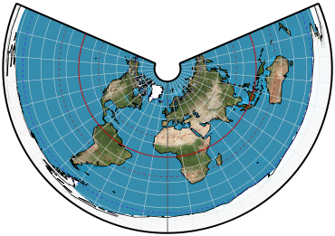
equidistant conic

simple conic

Parameters: Latitude of origin, Standard parallel 1, Standard parallel 2

Classifications

conic
equidistant

Graticule

Meridians: Equally spaced straight lines converging at a common point, which is normally beyond the pole. The angles between them are less than the true angles.
Parallels: Equally spaced concentric circular arcs centered on the point of convergence of the meridians, which are therefore radii of the circular arcs.
Poles: Normally circular arcs enclosing the same angle as that enclosed by the other parallels of latitude for a given range of longitude.
Symmetry: About any meridian.

Limiting forms

Polar azimuthal equidistant projection, if a pole is made the single standard parallel. The cone of projection thereby becomes a plane.
Plate Carree, if the single standard parallel is the equator. The cone of projection thereby becomes a cylinder.
Equirectangular (cylindric) projection, if two standard parallels are symmetrically placed north and south of the equator.
Standard conic formulas must be rewritten for the second and third limiting forms.

Scale

True along each meridian and along one or two chosen standard parallels, usually but not necessarily on the same side of the equator. As a rule of thumb, these parallels can be placed at one-sixth and five-sixths of the range of latitudes, but there are more refined means of selection. Scale is constant along any given parallel.

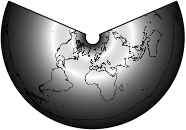
Distortion

Free of distortion only along the two standard parallels. Distortion is constant along any given parallel. Compromise in distortion between equal-area and conformal conic projections.

Usage

The most common projection in atlases for small countries.
Also used by the Soviet Union for mapping that nation.

Similar projections

Various methods of determining optimum standard parallels have been proposed by Patrick Murdoch (projections I, III) in 1758, Leonhard Euler in 1777, British Ordnance in the late 19th century, Dmitri I. Mendeleev in 1907, Wilhelm Schjerning (projection I) in 1882, V.V. Vitkovskiy (projection I) in 1907, and V.V. Kavrayskiy (projections II, IV) in 1934. Once the standard parallels are selected, all these projections are constructed by using formulas used for the equidistant conic with two standard parallels.
John Bartholomew combined the equidistant conic projection with the Bonne projection.

Origin

Rudimentary forms developed by Claudius Ptolemy (about A. D. 100).
Improvements by Johannes Ruysch in 1508, Gerardus Mercator in the late 16th century, and Nicolas de l'Isle in 1745.

Description adapted from J.P. Snyder and P.M. Voxland, An Album of Map Projections, U.S. Geological Survey Professional Paper 1453. United States Government Printing Office: 1989.